ASABE 2026 Student Robotics Challenge
Team
- Faculty Advisor: Dr. Vivian Vuong
- Graduate Advisors: Heesup Yun, Earl Ranario, Willian Klippel Huber, Zhian Li
- Undergraduate Members: Kaileen Navas, Madeleine Kim, Nico Puente, Serenity Pico
Links
GitHub Repository Hugging Face Dataset
We built a small autonomous field robot for the 2026 ASABE Student Robotics Challenge. It drives an 8 ft × 8 ft competition board, follows black guidelines, counts corn stands, and removes unhealthy yellow plants from double stands. The work was done at the UC Davis Department of Biological and Agricultural Engineering.
Why corn stand counting matters
Corn makes up more than 95% of total feed grain production and use in the U.S. Farmers check plant population, or “stand count,” to decide whether replanting is needed. Common methods such as the 1/1000th-acre, stick, or hoop methods are slow, require people in the field, and vary with who is counting. A small robot that can count stands automatically would save time and give more consistent numbers. If it can also remove unhealthy plants from crowded double stands, it helps the remaining healthy plant grow better.
What the robot needs to do
Our design targets four objectives:
- Autonomous navigation: follow straight and curved lines on the board and stop at each planting location.
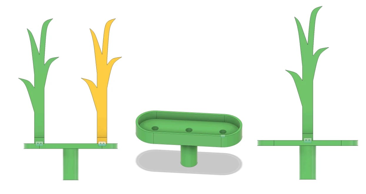
- Plant classification: tell the difference between a single healthy green plant, an empty spot, and a double stand with one green and one yellow plant.
- Selective actuation: knock down only the yellow plant in a double stand, leaving the green one alone.
- Integrated control: combine navigation, classification, and actuation into one reliable sequence.
Hardware
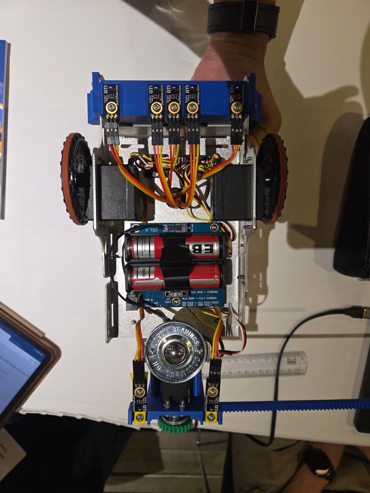
The base platform is the Parallax cyber:bot Robot Kit with a micro:bit v2. It has a differential drive with two independently powered wheels, so we can control forward speed and turning by varying the wheel speeds.
| Component | Role |
|---|---|
| Parallax cyber:bot + micro:bit | Chassis and main controller |
| Parallax QTI Line Follower AppKit | Four infrared sensors for black-line tracking |
| Parallax Ping))) Ultrasonic sensors | Distance checks near corners and stands |
| Pixy2 CMUcam5 | Color-based plant classification |
| Parallax Feedback 360° servo | Actuation rod for knocking down yellow plants |
| I2C LCD 1602 | Live status display during runs |
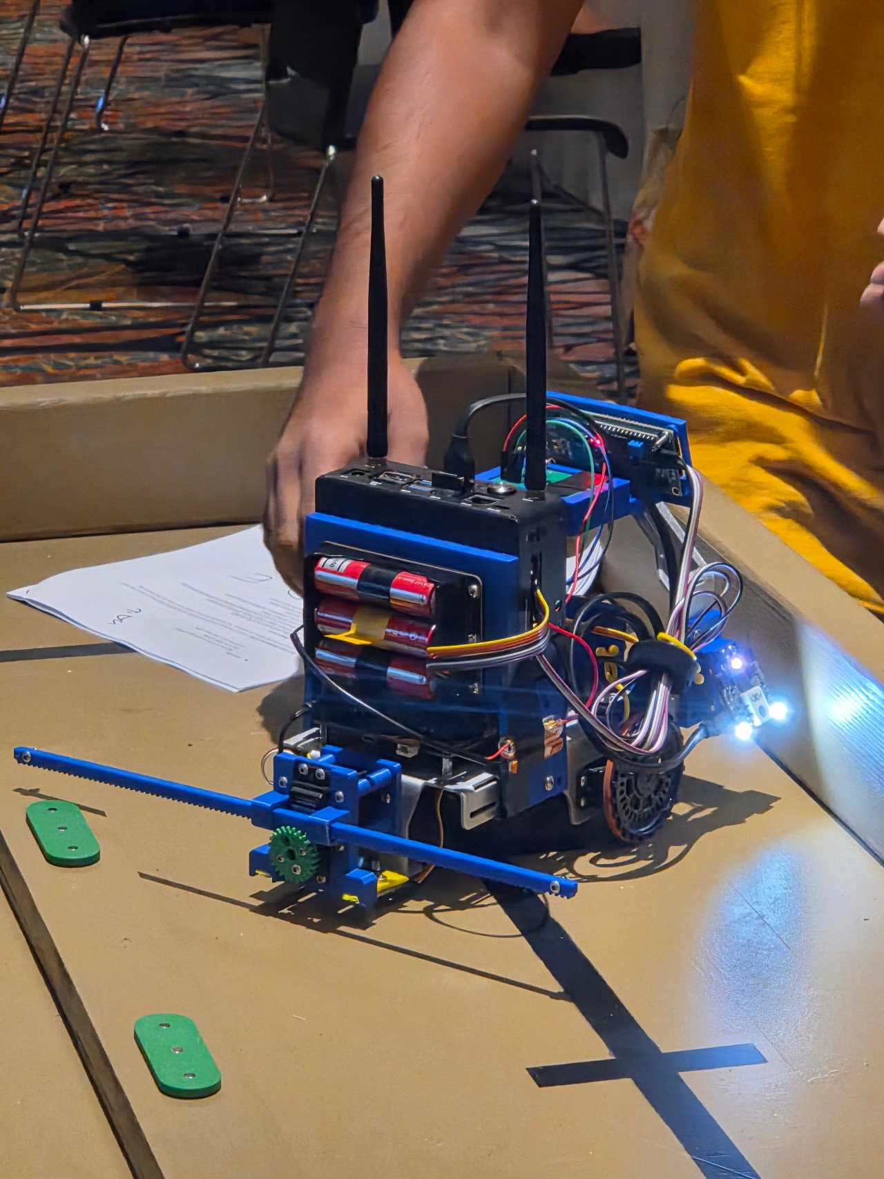
The servo drives a geared mechanism that extends and retracts a rod. When the Pixy2 sees a yellow plant in a double stand, the rod extends and the robot moves forward or backward just enough for the rod to hit the yellow plant. After that, the rod retracts and the robot continues.
Software architecture
The control code runs a 20 Hz Sense-Plan-Act loop. The same loop implementation in robot_loop.py is used by both the simulator and the physical micro:bit:
- Sense: read QTI line sensors and gyro/heading.
- Plan: update the EKF, pick the next waypoint command, compute motor speeds.
- Act: set left and right motor velocities.
- Sleep: wait for the next 50 ms cycle.
# robot_loop.py

def step(platform):
    nav = platform.get_navigation()

    qti = platform.read_qti()
    gyro = platform.read_gyro()
    nav.sense(qti_override=qti, gyro_override=gyro)

    if platform.has_cameras():
        nav.process_camera("L", platform.read_camera("L"))
        nav.process_camera("R", platform.read_camera("R"))

    nav.plan()
    vL, vR = nav.actuate()
    platform.set_motors(vL, vR)
    platform.update_display()
    platform.sleep()
This layout lets us tune navigation in simulation and then move the same logic to hardware with only the platform layer changing.
Navigation
We estimate the robot pose with an Extended Kalman Filter. The state vector is:
\[\mathbf{x}_k = \begin{bmatrix} x_k \\ y_k \\ \theta_k \end{bmatrix}\]From wheel velocities $v_L$ and $v_R$, the odometry prediction step is:
\[v_k = \frac{v_L + v_R}{2}, \quad \omega_k = \frac{v_L - v_R}{W}\] \[\mathbf{x}_k^- = \mathbf{x}_{k-1} + \begin{bmatrix} v_k \cos(\theta_{k-1}) \Delta t \\ v_k \sin(\theta_{k-1}) \Delta t \\ \omega_k \Delta t \end{bmatrix}\]where $W$ is the wheelbase and $\Delta t = 0.05$ s.
Because the micro:bit has limited flash and RAM, the EKF is written with inline scalar updates rather than a full matrix library. When the robot is on a line, the heading estimate is corrected toward the expected line direction. When it reaches a waypoint, the position snaps to the known coordinate and the covariance resets to small values.
Line following
The four QTI sensors report whether they are over the black line. We compute a lateral error with sensor weights $[-3, -1, 1, 3]$:
\[e_k = \frac{\sum_{i=0}^{3} s_{i,k} \, w_i}{\sum_{i=0}^{3} s_{i,k}}\]The derivative of this error is filtered with a first-order low-pass to reduce noise, then a PD controller sets the steering differential:
\[u_k = K_p e_k + K_d d_k\]The steering command is capped at 80% of the base speed to avoid overcorrection. The final wheel velocities are:
\[v_L = v_{\text{follow}} + u_k^{\text{sat}}, \quad v_R = v_{\text{follow}} - u_k^{\text{sat}}\]Mission path
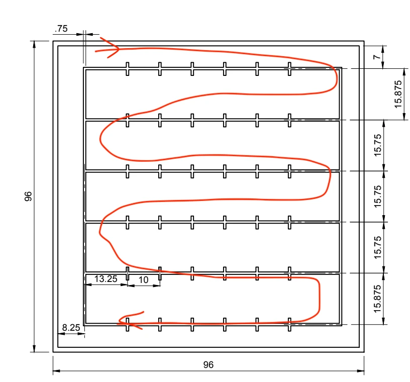
The board has five parallel sand beds. The robot follows a serpentine path generated by waypoint.py: it drives down one row, turns, drives back down the next, and repeats until it has visited every plant station. Each waypoint carries a command such as straight, detect left, detect right, turn clockwise, or finish.
Vision: YOLOv8 plant detection
The written report describes the Pixy2 color camera used in the original design. Alongside that, we trained a YOLOv8-based corn-plant detector for faster and more general classification. This part of the project is in camera/object_detection/.
Dataset
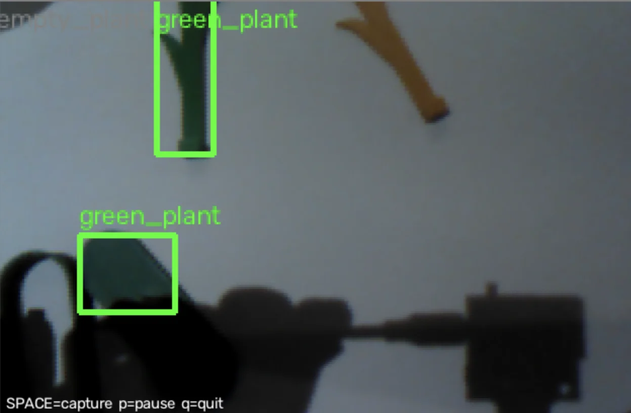
We collected 651 raw frames from the robot’s cameras, ran a pre-trained YOLOv8 person detector to remove any frames with people or body parts, and kept 213 clean images. Of those, 190 have bounding-box annotations. The public dataset is on Hugging Face:
Classes are green_plant and yellow_plant. COCO IDs are 1 and 2; YOLO IDs are 0 and 1.
Training pipeline
train_model.py runs the whole training workflow:
- Merge per-image LabelMe JSONs into a single COCO
annotations.json. - Convert COCO to Ultralytics YOLO format and split into train/val.
- Optionally augment the training split with
augment_dataset.py. - Train a YOLOv8 model (default
yolov8n.pt) at 320 × 320 resolution. - Export the best weights to ONNX.
- Copy
best.pt,best.onnx, anddata.yamlintomodels/<name>/.
Example:
python camera/object_detection/train_model.py \
    --name plant_detect_v5 --augment 3 --epochs 100
augment_dataset.py applies horizontal flip, brightness/contrast, HSV and RGB shifts, Gaussian noise, blur, shift/scale/rotate, and coarse dropout to improve robustness to lighting and camera jitter.
Inference
run_yolo.py supports three backends and automatically picks one from the file extension:
- PyTorch
.pt - ONNX Runtime
.onnx - TensorRT
.engine
It can run on a single image, a folder, a USB camera, or the Pixy2. By default it rotates the image 180° because our cameras are mounted upside-down on the robot.
Jetson Nano deployment
For real-time use on the robot’s Jetson Nano, export_jetson.py builds a TensorRT FP16 engine from the ONNX model. get_blocks_cpp_demo.py then runs dual Pixy2 cameras on the Jetson, classifies each frame, and updates an I2C LCD and status LEDs. When a yellow plant is detected in a double stand, it sends a single-character serial command to the micro:bit (0 for no action, 1 for forward knock, or 2 for backward knock), so the actuation can be triggered without slowing down the main control loop.
Simulation dashboard
Before running on hardware, we tested everything in a Python/Tkinter simulator. real2sim_main.py renders the board, the robot, the QTI sensor states, the camera field-of-view, and the live EKF covariance. The dashboard can also export the driven trajectory to CSV.
To make the simulation realistic, we added noise models:
- QTI sensors get spatial jitter and 2% random bit-flips.
- Servo motors get 2–10% bias plus Gaussian speed noise.
- Kinematic slip is applied to translation and rotation.
We ran 100 randomized missions. The robot completed all 100, with an average run time of about 145 s and a maximum path error around 8 inches.
The simulator below runs entirely in the browser. Press Start (Auto Mode) to run a mission, Reset to randomize the plant layout, or switch to manual mode and drive with WASD / arrow keys (on a phone, use the on-screen arrow buttons). Speed buttons run the physics faster without changing the simulation accuracy.
Micro:bit deployment
The micro:bit has strict flash and RAM limits, so deploy.py strips comments and docstrings, compresses indentation, and removes extra whitespace from the source files before copying them to the Mu Editor workspace. It also removes legacy .mpy files to prevent allocation errors. The deployed code includes main.py, config.py, cyberbot.py, ping.py, and QTI helpers.
Results and next steps
The robot met the main design goals in simulation: it navigates the full course, classifies stands, and actuates when needed. Future work is focused on real-world reliability: more testing under different lighting for the vision system, finer actuation alignment so the rod hits only the target plant, and adding wheel encoders or better heading feedback to reduce turning drift.